SPGL1: A Brief Tour

Michael P. Friedlander, June 2008

SPGL1 is a solver for one-norm regularized least-squares. It is suitable for problems that are large-scale and in the complex domain. This document gives a brief tour of SPGL1's main features.

Generate random data
Basis pursuit
Basis pursuit denoise
LASSO
Complex variables
The Pareto curve
Reference

Generate random data

The examples below are based on randomly generated data. We'll begin by creating a random m-by-n encoding matrix and a sparse solution vector:

rand('twister',0); randn('state',0);
m = 50; n = 128; k = 14;                   % No. of rows (m), columns (n), and nonzeros (k)
[A,Rtmp] = qr(randn(n,m),0);               % Random encoding matrix with orthogonal rows
A  = A';                                   % ... A is m-by-n
p  = randperm(n); p = p(1:k);              % Location of k nonzeros in x
x0 = zeros(n,1); x0(p) = randn(k,1);       % The k-sparse solution
b  = A*x0;                                 % The right-hand side corresponding to x0

Basis pursuit

The basis pursuit (BP) problem

  minimize ||x||_1  subject to  Ax = b

often finds the sparsest solution to the linear system of equations Ax = b. The call to SPGL1 is straightforward:

opts = spgSetParms('verbosity',0);         % Turn off the SPGL1 log output
x = spg_bp(A, b, opts);

Let's verify that the true sparse solution was recovered correctly:

plot(x0,'r*'); hold on
stem(x ,'b '); hold off
legend('Original coefficients','Recovered coefficients');
title('Basis Pursuit');

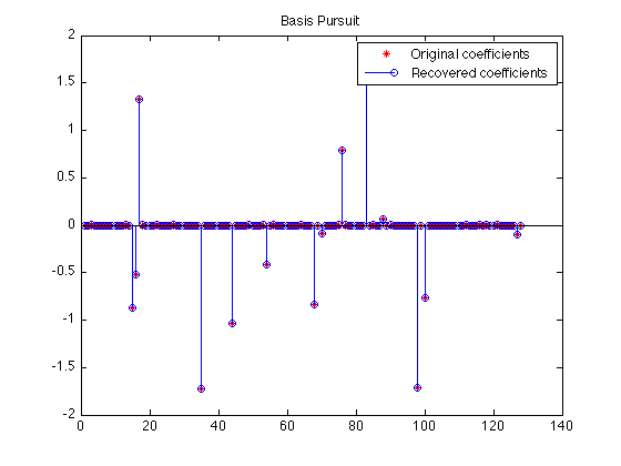
As a final check, the residual should be nearly zero:

norm(b - A*x)

ans =
   8.3531e-05

Basis pursuit denoise

If there was noise inherent in the signal that we measured, it would be better to instead solve the basis pursuit denoise (BPDN) problem

  minimize ||x||_1  subject to  ||Ax - b||_2 <= sigma,

which only approximately fits the equation Ax=b. In this experiment, we'll set sigma = 0.1:

b = A * x0 + randn(m,1) * 0.075;
sigma = 0.1;                                     % Desired ||Ax - b||_2
opts = spgSetParms('verbosity',0);
x = spg_bpdn(A, b, sigma, opts);

We don't expect the recovery to be exact this time because of the noise:

plot(x0,'r*'); hold on
stem(x ,'b '); hold off
legend('Original coefficients','Recovered coefficients');
title('Basis Pursuit Denoise');

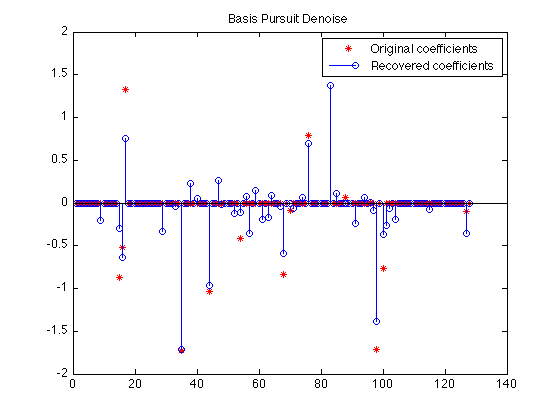
The corresponding residual should have a norm (nearly) equal to sigma (0.1):

norm(b - A*x)

ans =
    0.0999

LASSO

The Lasso problem puts a constraint directly on the one-norm of the solution:

  minimize ||Ax - b||_2  subject to  ||x||_1 <= tau

Here, we'll recover a least-squares solution with a one-norm equal to pi -- an easily recognizable number! We'll turn on SPGL1's output so that we can see it's progress:

opts = spgSetParms('verbosity',1);
tau = pi;
x = spg_lasso(A, b, tau, opts);

 ================================================================================
 SPGL1  v. 1017  (Mon, 16 Jun 2008)
 ================================================================================
 No. rows              :       50      No. columns           :      128
 Initial tau           : 3.14e+00      Two-norm of b         : 2.61e+00
 Optimality tol        : 1.00e-04      Target one-norm of x  : 3.14e+00
 Basis pursuit tol     : 1.00e-06      Maximum iterations    :      500

  Iter      Objective   Relative Gap      gNorm   stepG    nnzX    nnzG
     0  2.6116134e+00  8.8203906e-01   9.57e-01     0.0       0       0
     1  1.7351041e+00  1.5596782e-01   5.16e-01     0.0      10       1
     2  1.7035044e+00  3.5470990e-02   4.43e-01     0.0       6       1
     3  1.6985890e+00  1.0356556e-02   4.16e-01     0.0       6       1
     4  1.6984830e+00  1.3137969e-03   4.09e-01     0.0       6       3
     5  1.6984820e+00  3.5582204e-04   4.09e-01     0.0       6       6
     6  1.6984819e+00  2.5425067e-05   4.09e-01     0.0       6       6

 EXIT -- Optimal solution found

 Products with A     :       7        Total time   (secs) :     0.0
 Products with A'    :       7        Project time (secs) :     0.0
 Newton iterations   :       0        Mat-vec time (secs) :     0.0
 Line search its     :       0        Subspace iterations :       0

The one-norm of the solution:

norm(x,1)

ans =
    3.1416

Complex variables

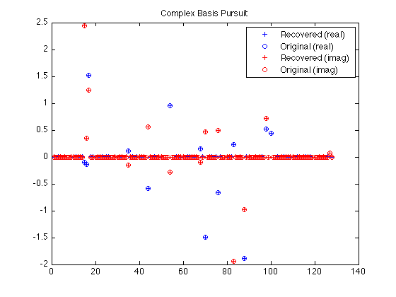
Many signal-processing problems involve complex-valued coefficients. In this example, we create a solution that is sparse in the Fourier domain. We simulate missing data by randomly restricting the rows of the Fourier operator. The resulting BP problem is

 minimize  ||z||_1  subject to  R*F*z = R*b,

where R is a restriction operator and F is a Fourier operator. Keep in mind that z is a complex variable, and that

 ||z||_1 = sum_j ( sqrt( x_j^2 + y_j^2 ) ), where z_j = x_j + i*y_j.

We use the partial Fourier operator

 z = partialFourier(idx,n,x,mode);

the index set idx

idx = randperm(n); idx = idx(1:m);

determines which rows of the Fourier operator are kept. We create an operator that conforms to SPGL1's requirements:

opA = @(x,mode) partialFourier(idx,n,x,mode);  % This is now "A"

Create sparse coefficients and the right-hand side b:

z0 = zeros(n,1);
z0(p) = randn(k,1) + sqrt(-1) * randn(k,1);
Rb = opA(z0,1);                                 % Rb = R*A*z0

Fire up SPG_BP in the usual way. Note that in this, case, the first argument is a function:

opts = spgSetParms('verbosity',0);
z = spg_bp(opA,Rb,opts);

Plot the recovered and original coefficients:

plot(1:n,real(z),'b+',1:n,real(z0),'bo', ...
     1:n,imag(z),'r+',1:n,imag(z0),'ro');
legend('Recovered (real)', 'Original (real)', ...
       'Recovered (imag)', 'Original (imag)');
title('Complex Basis Pursuit');

The Pareto curve

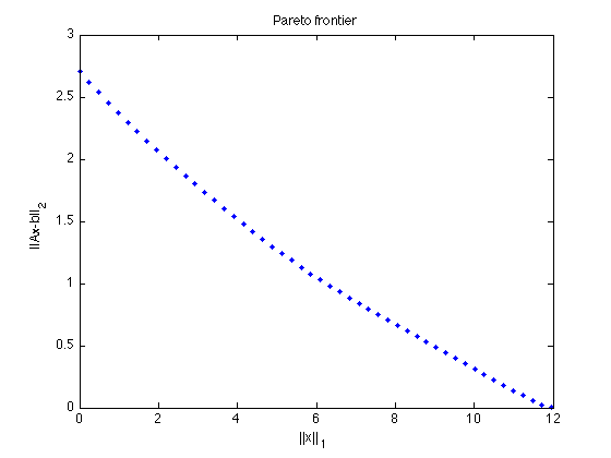
The Pareto curve traces the optimal tradeoff between the one-norm of the solution and the two-norm of the residual. We take advantage here of SPGL1's warm-start capability and sample the Pareto curve at a bunch of points.

We do this by solving a sequence of LASSO problems for increasing values of tau. Larger values of tau will yield smaller residuals. In fact, if phi(tau) is the norm of the residual corresponding to a given tau, then phi is a continuously differentiable function [BergFriedlander08].

Because here we wish to warm-start SPGL1, we need to use its expert interface, rather than the simpler interface available via SPG_LASSO.

b = A*x0;
tau = linspace(0,1.01*norm(x0,1),50);      % Values of tau at which to sample
phi = zeros(size(tau));                    % Preallocate the vector of residuals.
x = zeros(n,1);                            % Initialize the solution.
opts = spgSetParms('verbosity',0);
for i=1:length(tau)
    [x,r] = spgl1(A,b,tau(i),[],x,opts);   % Re-solve LASSO(tau) with a different tau.
    phi(i) = norm(r,2);                    % SPGL1's 2nd output arg is the residual.
end

Plot the curve.

plot(tau,phi,'b.');
title('Pareto frontier');
xlabel('||x||_1'); ylabel('||Ax-b||_2');

Reference

[BergFriedlander] E. van den Berg and M. P. Friedlander, "Probing the Pareto frontier for basis pursuit solutions", January 2008 (revised May 2008). To appear in SIAM Journal on Scientific Computing.

% $Id: spgexamples.m 1077 2008-08-20 06:15:16Z ewout78 $