Least Squares

Linear least-squares, also known as ordinary linear regression, is a basic optimization problem used for data fitting. It's also a fundamental building block for algorithms meant for more general problems.

Example: Multilinear regression

We begin with a simple example and use linear regression to build a model that relates the fuel efficiency of a car with its weight, engine displacement, and engine horsepower. Load the mtcars dataset provided in the Rdatasets.jl package:

using RDatasets
mtcars = RDatasets.dataset("datasets", "mtcars")

Here are the first five rows of the dataset, which contains 32 rows in total:

first(mtcars, 5)

5×12 DataFrame
 Row │ Model              MPG      Cyl    Disp     HP     DRat     WT       QSec     VS     AM     Gear   Carb
     │ String31           Float64  Int64  Float64  Int64  Float64  Float64  Float64  Int64  Int64  Int64  Int64
─────┼──────────────────────────────────────────────────────────────────────────────────────────────────────────
   1 │ Mazda RX4             21.0      6    160.0    110     3.9     2.62     16.46      0      1      4      4
   2 │ Mazda RX4 Wag         21.0      6    160.0    110     3.9     2.875    17.02      0      1      4      4
   3 │ Datsun 710            22.8      4    108.0     93     3.85    2.32     18.61      1      1      4      1
   4 │ Hornet 4 Drive        21.4      6    258.0    110     3.08    3.215    19.44      1      0      3      1
   5 │ Hornet Sportabout     18.7      8    360.0    175     3.15    3.44     17.02      0      0      3      2

The model that we wish to build aims to find coefficients $x_1,\ldots,x_4\in\mathbb R$ such that for each particular car model $i=1,2,\ldots,32$,

Of course, we shouldn't expect an exact match for all car models $i$, and instead the coefficients $x_1,\ldots,x_4$ computed by ordinary linear regression minimizes the sum of least-squares deviations:

$$\min_{x_1,\ldots,x_4}\ \sum_{i=1}^{32} (x_1 + x_2\cdot\text{Disp}_i + x_3\cdot\text{HP}_i + x_4\cdot\text{WT}_i - \text{MPG}_i)^2$$

Because this is such an important problem in general, there exists excellent software packages that make formulating and solving these problems easy. Here's how to do it using the generalized linear models package GLM.jl:

using GLM
ols = lm(@formula(MPG ~ Disp + HP + WT), mtcars)

StatsModels.TableRegressionModel{GLM.LinearModel{GLM.LmResp{Vector{Float64}}, GLM.DensePredChol{Float64, LinearAlgebra.CholeskyPivoted{Float64, Matrix{Float64}, Vector{Int64}}}}, Matrix{Float64}}

MPG ~ 1 + Disp + HP + WT

Coefficients:
───────────────────────────────────────────────────────────────────────────────
                    Coef.  Std. Error      t  Pr(>|t|)   Lower 95%    Upper 95%
───────────────────────────────────────────────────────────────────────────────
(Intercept)  37.1055        2.11082    17.58    <1e-15  32.7817     41.4293
Disp         -0.000937009   0.0103497  -0.09    0.9285  -0.0221375   0.0202635
HP           -0.0311566     0.0114358  -2.72    0.0110  -0.0545817  -0.00773139
WT           -3.80089       1.06619    -3.56    0.0013  -5.98488    -1.6169
───────────────────────────────────────────────────────────────────────────────

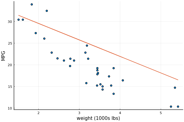
The column marked Coef. shows the values for the 4 computed coefficients $x_1,\ldots,x_4$; the remaining columns show the results for various statistical tests that indicate the reliability of each coefficient It appears that the car's weight has the biggest impact on fuel economy. This plot shows the projection of the data and the regression line onto the plane spanned by WT and MPG:

using StatsPlots; pyplot()
x₁, x₄ = coef(ols)[[1,4]]
@df mtcars scatter(:WT, :MPG, xlabel="weight (1000s lbs)", ylabel="MPG", leg=false)
@df mtcars plot!(:WT, x₁ .+ x₄*:WT)

Matrix formulation

The objective (1) can be written using matrix notation, as follows: define the matrix and vector

where $m=32$. Thus, the least-squares soluition $x^*$ minimizes the 2-norm squared $\|r\|^2$ of the residual $r = b - Ax$.

General least-squares formulation

The general linear-least squares problem is formulated as

$$\min_{x\in\mathbb R^n}\ \tfrac12\|r\|^2, \quad r = b - Ax,$$

where $A$ is an $m$-by-$n$ matrix, $b$ is an $m$-vector, $x$ is an $n$-vector, and $r$ is an $m$-vector of residuals. Typically, there are many more observations than $m$ than variables $n$, and so $m\gg n$. But there are many important application that require least-squares problems where the opposite is true – these problems are considered under determined because there are necessarily infinitely many least-squares solutions $x_\mathrm{\tiny LS}.$

The following fundamental result describes several equivalent conditions that any least-squares solution must satisfy.

This result relies on a fundamental property that for all matrices $A$, regardless of their shape, the subspaces

are orthogonal complements, i.e.,

The equivalence of the three properties is then straightforward, and it's sufficient to show that the third condition is equivalent to the optimality of the least-squares problem. Orthogonally decompose the residual $r = b-y$ as

If $y$ was not the orthogonal projection of $b$, then there must exist some component of $b-y$ in the range of $A$. Thus, $z_r\ne0$ and

which means we found a new point $(y+z_r)\in\hbox{range}(A)$ with a smaller residual, which contradicts the optimality of $x_\mathrm{\tiny LS}$, and also the uniqueness of the projection $y$.

Example: Multilinear regression (continued)

For the multilinear regression example, we can obtain the least-squares solution by solving the normal equations as follows:

using LinearAlgebra # gives `norm` function
A = [ones(size(mtcars,1)) mtcars[:,:Disp]  mtcars[:,:HP] mtcars[:,:WT]]
b = mtcars[:,:MPG]
x = A'A \ A'b
@show(norm(x-coef(ols)))

norm(x - coef(ols)) = 2.1871395004271944e-14

The coefficients computed using the normal equations are almost the same as those computed using by GLM, which likely solves the normal equations using a different method.

The least-squares solution should also verify the first condition of the above theorem:

r = b - A*x
@show(norm(A'r))

norm(A' * r) = 6.115154620218894e-11

The backslash operator

In this last example, we solved for the least-squares solution by explicitly solving the normal equations $A^T\! Ax=A^T\! b$ via the Julia command x = A'A \ A'b. As we'll see in a later lecture, this isn't the best way to solve the least-squares problem. Without getting into the details just yet, it's enough for now to know that Julia allows for the short-hand x = A \ b: Julia recognizes that this is an overdetermined system, and solves for the least-squares solution using a mathematically equivalent approach. Let's verify:

x1 = A \ b
@show norm(x1 - x, Inf)

norm(x1 - x, Inf) = 4.334310688136611e-13

Close enough!

Example: Trendline

This example uses least-squares to illustrate the increasing concentrations of nitrous oxide (N₂O), which is a greenhouse gas. We'll use a dataset from the Global Monitoring Laboratory:

fname = "mlo_N2O_All.dat"
if !isfile(fname)
	download("https://gml.noaa.gov/aftp/data/hats/n2o/insituGCs/CATS/hourly/mlo_N2O_All.dat", fname)
end

This dataset provides hourly measurements of N₂O levels in parts per billion (ppb) from 1999 to 2021 from gas sampled at the Manua Loa Observatory in Hawaii. The following code removes rows with missing concentration levels ppb, and creates a new table with average monthly measurements:

using CSV, DataFrames, DataFramesMeta, Statistics
df = CSV.read(fname, DataFrame, comment="#", normalizenames=true, delim=" ", ignorerepeated=true)
dfg = @chain df begin
    @select(:year = :N2OcatsMLOyr, :month = :N2OcatsMLOmon, :ppb = :N2OcatsMLOm)
    @subset((!isnan).(:ppb))
    @by([:year, :month], :avgppb = mean(:ppb))
end 
describe(dfg, :min, :max, cols=[:year, :avgppb])

2×3 DataFrame
 Row │ variable  min      max
     │ Symbol    Real     Real
─────┼─────────────────────────────
   1 │ year      1999     2022
   2 │ avgppb     315.06   337.484

A trend line is defined by the univariate function

where $\alpha$ is the intercept, $\beta$ is the slope, and $t$ is time. Here, we'll just index the months by the integers $t=1,2,\ldots,T$. We determine the parameters $\alpha$ and $\beta$ by solving the least-squares problem

which corresponds to the general least-squares problem with

In Julia,

T = nrow(dfg)
t = collect(1:T)
A = [ones(T)  t]
b = dfg[!, :avgppb]

The least-squares solution is then

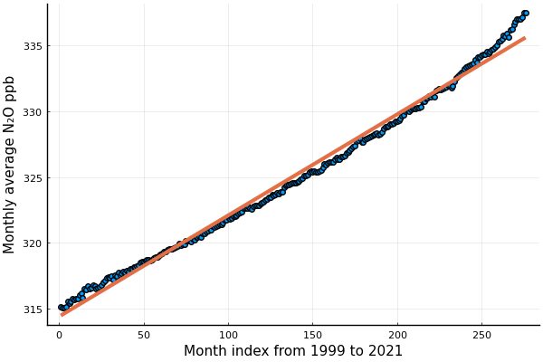
α, β = A \ b

and we can plot the data together with the trend line:

@df dfg scatter(:avgppb) 
p(t) = α + β*t
plot!(p, lw=3)
plot!(leg=false, xlab="Month index from 1999 to 2021", ylab="Monthly average N₂O ppb")

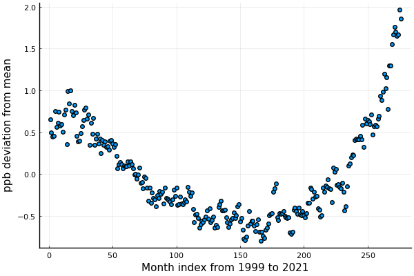
But perhaps most interestingly, we can now "detrend" the data to understand how the concentrations vary around the overall 22-year trend:

@df dfg scatter(:avgppb - p.(t))