Nonlinear Least-Squares

The nonlinear least-squares problem generalizes the linear least-squares problem to include nonlinear residual functions. The Gauss-Newton solves this problem as a sequence of least-squares subproblems.

Nonlinear residuals

The nonlinear least squares problem seeks to minimize the sum of squares

$$\min_{x\in\mathbb R^n}\ \tfrac12\|r(x)\|^2,$$

where the $m$-vector of residuals

is composed of differentiable nonlinear functions $r_{i}:\mathbb R^n→\mathbb R$. The non-linear least squares problem reduces to linear least-squares when $r$ is affine, i.e., $r(x) = Ax-b$ for some $m$-by-$n$ matrix $A$ and $m$-vector of observations $b$.

Linearizing the residual

We can solve non-linear least squares problem (1) by solving a sequence of linear least-squares problem, which result from linearization of $r$ at the current estimate of the ground truth $x$.

The linear approximation of $r$ at a point $x^k \in \mathbb R^n$ is defined by

where

$$J(x) = \begin{bmatrix} \nabla r_1(x)^T\\ \vdots \\ \nabla r_m(x)^T\end{bmatrix}$$

is the Jacobian of $r$ evaluated at $x$

If the linesearch parameter $\alpha$ is held fixed at 1, then this is a "pure" Gauss-Newton iteration. We'll later discuss options for when it's advisable to use smaller steps.

Here's a basic version of the method that takes as arguments the residual and Jacobian functions r and J, and a starting vector x.

function gauss_newton(r, J, x; ε=1e-4, maxits=30)
  err = []
  for i = 1:maxits
      rk, Jk = r(x), J(x)
      push!(err, norm(Jk'rk))
      err[end] ≤ ε && break
      x = x - Jk\rk 
    end
    return x, err
end

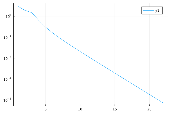
The condition err[end] ≤ ε causes the iterations to terminate when the latest residual rk is nearly orthogonal to all the gradients of the residual, i.e., the residual is orthogonal to the tangent space of the level-set for the nonlinear least-squares objective $\tfrac12\|r(x)\|^2$. This is exactly analogous to the optimality condition for linear least-squares.

Example: Position estimation from ranges

Let $x \in \mathbb R^2$ represent the unknown position of an object. Our aim is to find the position of this object relative to a set of $m$ beacons placed in fixed known positions $b_{i} \in \mathbb R^2$, $i = 1,\dots,m$. The only data available are range measurements $δ_i$ that give an estimate of the distance between each beacon $b_{i}$ and the object at $x$, i.e.,

$$δ_i := \| x-b_i\| + ν_i$$

where each scalar $ν_i$ represents the error between the true (and unkown) distance $\| x-b_i\|$ and the measurement $δ_i$.

We can obtain an estimate of the object's position $x$ by solving the nonlinear least-squares problem (1) where we define the $i$th residual between the reported distance $δ_i$ and the distance between the position $b_i$ of the $i$th beacon and $x$:

Here's the residual function, which takes a vector of ranges $δ$ and a vector of positions b:

r(x, δ, b) = [ δ[i] - norm(x - b[:,i]) for i in 1:length(δ) ]

Use the following Julia packages for this example.

using Random
using Statistics
using LinearAlgebra
using ForwardDiff
using Plots

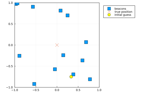
We simulate data by placing m beacons in random locations:

m = 13                 # number of beacons
b = 2rand(2, m) .- 1   # place beacons uniformly in the unit box 
x = zeros(2)           # true position 
x0 = 2rand(2) .- 1     # initial guess of the unknown position
ν = .5*rand(m)
δ = [ norm(x - b[:,i]) + ν[i] for i in 1:m]

Place these items on a map (we'll wrap this in a function so that we can reuse it below):

function plotmap(b, x, x0)
scatter(xlim=(-1,+1), ylim=(-1,+1), leg=:outertopright,frame=:box, aspect_ratio=:equal)
scatter!(b[1,:], b[2,:], label="beacons", shape=:square, ms=7)
scatter!(x[1,:], x[2,:], label="true position", shape=:xcross, ms=7)
scatter!(x0[1,:], x0[2,:], label="initial guess", c="yellow", ms=7)
end
plotmap(b, x, x0)

J(x) = ForwardDiff.jacobian(x->r(x, δ, b), x)
xs, err = gauss_newton(x->r(x, δ, b), J, x0)
plot(err, yaxis=:log)

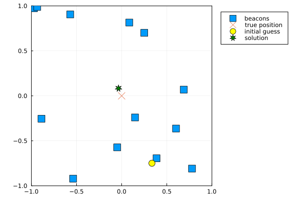
Plot the original map and overlay the obtained solution:

plotmap(b, x, x0)
scatter!(xs[1,:], xs[2,:], label="solution", shape=:star7, c="green", ms=7)