Gradients
Gradients provide information on a function’s sensitivity to perturbations in the input.
Slides
Directional derivatives
The behavior of a function \(f:\R^n\to\R\) along the ray \(\{x+αd\mid α\in\R_+\}\), where \(x\) and \(d\) are \(n\)-vectors, is given by the univariate function \[ \phi(\alpha) = f(x+αd). \] From standard calculus, the derivative of \(\phi\) at the origin, when it exists, is the limit \[ \phi'(0) = \lim_{α\to0^+}\frac{\phi(α)-\phi(0)}{α}. \] We thus arrive at the following definition.
Definition 1 (Directional derivative) The directional derivative of a function \(f:\R^n\to\R\) at a point \(x\in\R^n\), along a direction \(d\in\R^n\), is the limit \[ f'(x;d) = \lim_{α\to0^+}\frac{f(x+αd)-f(x)}{α}. \]
It follows immediately from this definition that the partial derivatives of \(f\) are simply the directional derivatives of \(f\) along the each of the canonical unit direction \(e_1,\ldots,e_n\), i.e., \[ \label{eq:partial-derivative} \frac{\partial f}{\partial x_i}(x) \equiv f'(x;e_i). \tag{1}\]
Descent directions
A nonzero vector \(d\) is a descent direction of \(f\) at \(x\) if the directional derivative is negative: \[ f'(x;d) < 0. \tag{2}\] It follows directly from the definition of the directional derivative that \(f(x+αd) < f(x)\) for all positive \(\alpha\) small enough.
Gradient vector
The gradient of the function \(f\) is the collection of all the partial derivatives: \[ \nabla f(x) = \begin{bmatrix} \frac{\partial f}{\partial x_1}(x) \\\vdots \\\frac{\partial f}{\partial x_n}(x) \end{bmatrix}. \] The gradient and directional derivative are related via the formula \[ f'(x;d) = \nabla f(x)\T d. \] If, for example, the direction \(d\) to be the canonical unit direction \(e_i\), then this formula reduces to \[ f'(x;e_i) = \nabla f(x)\T e_i = [\nabla f(x))]_i = \frac{\partial f}{\partial x_i}(x), \] which confirms the identity Equation 1.
Linear approximation
The gradient of a continuously differentiable function \(f\) (i.e., \(f\) is differentiable at all \(x\) and \(\nabla f\) is continuous) provides a local linear approximation of \(f\) in the following sense: \[ f(x+d) = f(x) + \nabla f(x)\T d + \omicron(\norm{d}), \] The residual \(\omicron:\R_+\to\R\) of the approximation decays faster than \(\norm{d}\), i.e., \[\lim_{α\to0+}\omicron(α)/α=0.\]
Example
Fortunately, there are good computational tools that automatically produce reliable gradients. Consider the 2-dimensional Rosenbrock function and its gradient: \[ \begin{align*} f(x) &= (a - x_1)^2 + b(x_2 - x_1^2)^2 \\ \nabla f(x) &= \begin{bmatrix} -2(a-x_1)-4b(x_2-x_1^2)x_1 \\ 2b(x_2-x_1^2) \end{bmatrix}. \end{align*} \]
Here is the code for \(f\) and its gradient:
Instead of computing gradients by hand, as we did above, we can use automatic differentiation, such as implemented in the package ForwardDiff, to compute these.
The function ∇fad returns the value of the gradient at x. Let’s compare the hand-computed gradient ∇f against that automatically-computed gradient ∇fad at a random point:
Calculus rules
We derive calculus rules for linear and quadratic functions, which appear often in optimization.
Linear functions
Let \(a\in\R^n\). The linear function \[ f(x) = a\T x = \sum_i^n a_i x_i \] has the gradient \(\nabla f(x) = a\), and so the gradient is constant. Here’s a small example:
Quadratic functions
Let \(A\in\R^{n\times n}\) be a square matrix. Consider the quadratic function \[ f(x) = \half x\T A x. \tag{3}\] One way to derive the gradient of this function is to write out the quadratic function making explicit all of the coefficients in \(A\). Here’s another approach that uses the product rule: \[ \begin{align*} ∇f(x) = \half ∇(x\T a) + \half ∇(b\T x), \end{align*} \] where \(a = Ax\) and \(b:=A\T x\) are held fixed when applying the gradient. Because each of the functions in the right-hand side of this sum is a linear function, we can apply the calculus rule for linear functions to deduce that \[ ∇f(x) = \half Ax + \half A\T x = \half (A+A\T)x. \] (Recall that \(A\) is square.) The matrix \(\half(A+A\T)\) is the symmetric part of \(A\). If \(A\) is symmetric, i.e., \(A = A\T\), then the gradient reduces to \[ ∇f(x) = Ax. \]
But in optimization, we almost always assume that the matrix that defines the quadratic in Equation 3 is symmetric because always \(x\T Ax = \half x\T(A+A\T)x\), and therefore we can instead work with the symmetric part of \(A\).
Example (2-norm). Consider the two functions \[ f_1(x) = \norm{x}_2 \quad\text{and}\quad f_2(x) = \half\norm{x}_2^2. \] The function \(f_2\) is of the form Equation 3 with \(A=I\), and so \(\nabla f_2(x) = x\). Use the chain rule to obtain the gradient of the \(f_1\): \[ \nabla f_1(x) = \nabla (x\T x)^\half = \half (x\T x)^{-\half}\nabla (x\T x) = \frac{x}{\norm{x}_2}, \] which isn’t differentiable at the origin.
Visualizing gradients
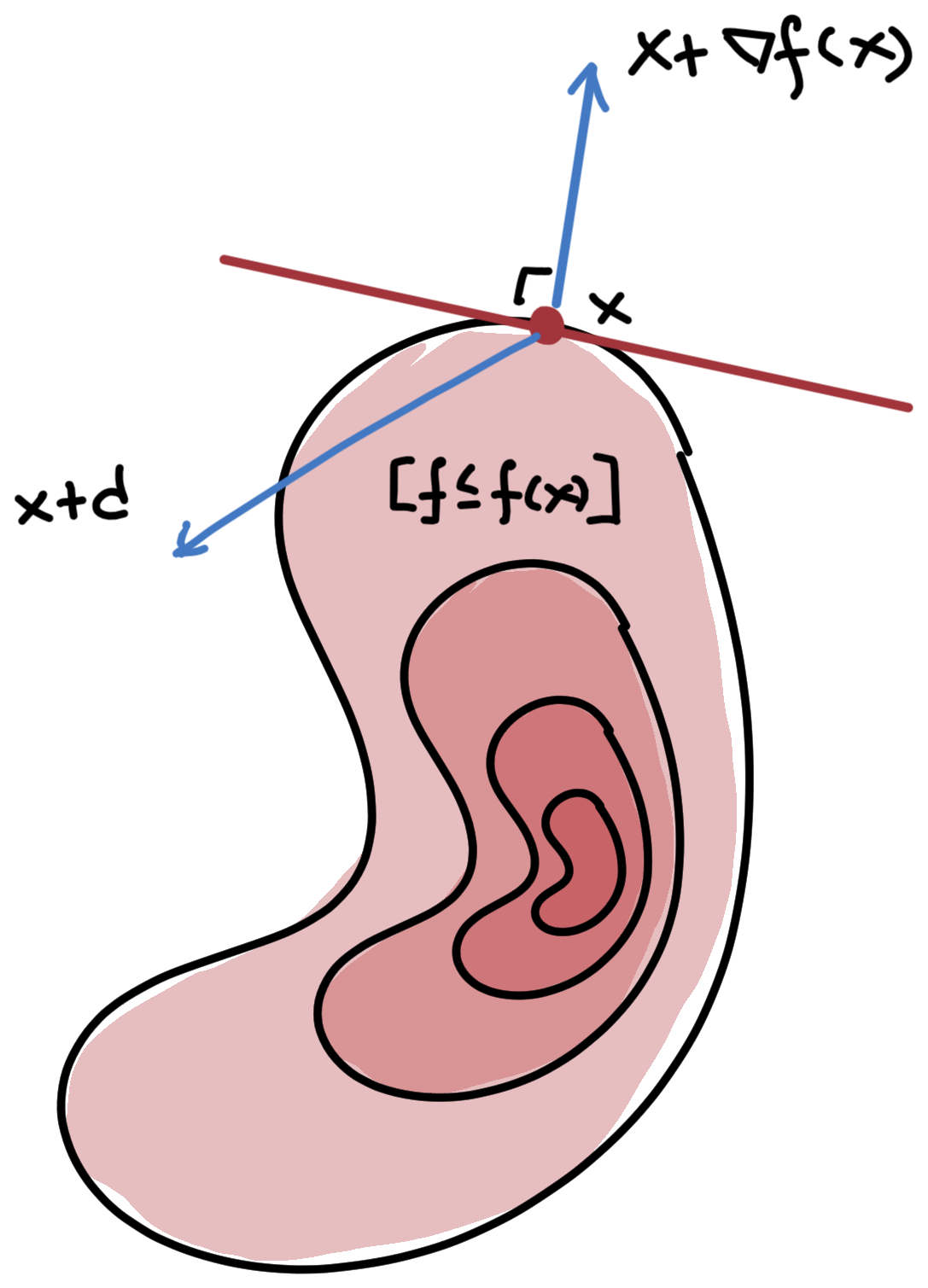
Gradients can be understood geometrically in relation to the level-set of the function. The \(α\)-level set of a function \(f:\R^n\to\R\) is the set of points that have an equal or lower value at \(x\): \[ [f≤α] = \{x\in\Rn\mid f(x)≤α\}. \] Fix any \(x\) and consider the level set \([f≤f(x)]\). For any direction \(d\) that’s either a descent direction for \(f\) or a tangent direction for \([f≤f(x)]\), \[ f'(x;d) = ∇f(x)\T d ≤ 0, \] which implies that the gradient \(\nabla f(x)\) is the outward normal to the level set, as shown in Figure 1.
