Gradients
Linearizations
Optimality

CPSC 406 – Computational Optimization

Gradients, linearizations, and optimality

\[ \def\argmin{\operatorname*{argmin}} \def\Ball{\mathbf{B}} \def\bmat#1{\begin{bmatrix}#1\end{bmatrix}} \def\Diag{\mathbf{Diag}} \def\half{\tfrac12} \def\ip#1{\langle #1 \rangle} \def\maxim{\mathop{\hbox{\rm maximize}}} \def\maximize#1{\displaystyle\maxim_{#1}} \def\minim{\mathop{\hbox{\rm minimize}}} \def\minimize#1{\displaystyle\minim_{#1}} \def\norm#1{\|#1\|} \def\Null{{\mathbf{null}}} \def\proj{\mathbf{proj}} \def\R{\mathbb R} \def\Rn{\R^n} \def\rank{\mathbf{rank}} \def\range{{\mathbf{range}}} \def\span{{\mathbf{span}}} \def\st{\hbox{\rm subject to}} \def\T{^\intercal} \def\textt#1{\quad\text{#1}\quad} \def\trace{\mathbf{trace}} \]

  • directional derivatives
  • gradients
  • first-order expansions
  • necessary conditions for optimality

Optimality

\[ \min_x\, f(x) \quad\text{where}\quad f:\Rn\to\R \]

\(x^*\in\Rn\) is a

  • global minimizer if \(f(x^*)\leq f(x)\) for all \(x\)
  • strict global minimizer if \(f(x^*)< f(x)\) for all \(x\)
  • local minimizer if \(f(x^*)\leq f(x)\) for all \(x\in\epsilon\Ball(x^*)\)
  • strict local minimizer if \(f(x^*)< f(x)\) for all \(x\in\epsilon\Ball(x^*)\)

Maximizers

  • flip inequalities for analogous maximizer def’s
  • \(\displaystyle\argmin_x \{f(x)\}=\argmax_x \{-f(x)\}\)

Optimal attainment

  • an optimal value may not be attained, eg,

    • \(\displaystyle\inf_x\, e^{-x}\) is not attained for any \(x\in\R\)
  • an optimal value may not exist, eg,

    • \(\displaystyle\min_x\, -x^2\) has no minimizer (unbounded below)
  • global solution set (may be empty, may have many elements)

    \[\argmin_x f(x) = \{\bar x\mid f(\bar x) \le f(x) \text{ for all } x\}\]

  • optimal values are unique even if an optimal point is not unique

Theorem 1 (Coercivity implies existence of minimizer) If \(f:\Rn\to\R\) is continuous and \(\lim_{\|x\|\to\infty}f(x)=\infty\) (coercive), then \(\min_x\, f(x)\) has a global minimizer.

Example

\[ \min_{x\in\R^2}\, \frac{x_1+x_2}{x_1^2+x_2^2+1} \]

  • global minimizer at \(-\frac{1}{\sqrt 2}(1,1)\)
  • global maximizer at \(\phantom-\frac{1}{\sqrt 2}(1,1)\)

(n=1)
scalar variable

Local optimality (1-D)

Let \(f:\R\to\R\) be differentiable. The point \(x=x^*\) is a

  • local minimizer if \[ \underbrace{f'(x) = 0}_{\text{stationary at $x$}} \textt{and} \underbrace{f''(x) > 0}_{\text{(strictly) convex at $x$}} \]

  • local maximizer if \[ \underbrace{f'(x) = 0}_{\text{stationary at $x$}} \textt{and} \underbrace{f''(x) < 0}_{\text{(strictly) concave at $x$}} \]

  • if \(f'(x)=0\) and \(f''(x)=0\), not enough information, eg,

    • \(f(\bar x)=x^3\) \(\quad\Longrightarrow\quad\) \(x=0\) in not a local minimizer or maximizer even though \(f'(0)=0\)
    • \(f(\bar x)=x^4\) \(\quad\Longrightarrow\quad\) \(x=0\) is the unique global minimizer even though \(f''(0)=0\)

Local optimality (1-D): motivation

  • suppose that at some \(x^*\), \(f'(x^*)=0\) and \(f''(x^*)>0\)
  • Taylor series, where remainder term \(\omicron(\alpha)/\alpha\to0\) as \(\alpha\to0^+\):

\[ f(x^*+\Delta x) = f(x^*) + \underbrace{f'(x^*)\Delta x}_{=0} + \underbrace{\tfrac{1}{2}f''(x^*)(\Delta x)^2}_{>0} + \omicron((\Delta x)^2) \]

  • divide both sides by \((\Delta x)^2\), and for \(\Delta x\) small enough, right-hand side is positive:

\[ \frac{f(x^*+\Delta x) - f(x^*)}{(\Delta x)^2} = \tfrac{1}{2}f''(x^*)+ \frac{\omicron((\Delta x)^2)}{(\Delta x)^2} > 0 \]

  • implies that \(f(x^*+\Delta x) > f(x^*)\) for \(\Delta x\) small enough

(n>1)
multivariable

Directional derivative

Restriction to a ray

restrict \(f:\Rn\to\R\) to the ray \(\{x+\alpha d\mid \alpha\in\R_+\}\): \[ \phi(\alpha) = f(x+\alpha d) \qquad \phi'(0) = \lim_{\alpha\to 0^+}\frac{\phi(\alpha)-\phi(0)}{\alpha} \]

Definition 1 The directional derivative of \(f:\R^n\to\R\) at \(x\in\R^n\) in the direction \(d\in\R^n\) is \[ f'(x;d) = \lim_{α\to0^+}\frac{f(x+αd)-f(x)}{α}. \]

partial derivatives are directional derivatives along each canonical basis vector \(e_i\): \[ \frac{\partial f}{\partial x_i}(x) = f'(x;e_i) \quad\text{with}\quad e_i(j) = \begin{cases} 1 & j=i\\ 0 & j\ne i\end{cases} \]

Descent directions

A nonzero vector \(d\) is a descent direction of \(f\) at \(x\), ie,

\[ f(x+\alpha d) < f(x) \quad \forall \alpha \in (0, \epsilon) \text{ for some } \epsilon > 0 \qquad(1)\]

equivalently, the directional derivative is negative:

\[ \begin{aligned} f'(x;d) := \lim_{\alpha\to 0^+}\frac{f(x+\alpha d)-f(x)}{\alpha} < 0 \end{aligned} \]

Gradients

If \(f:\Rn\to\R\) is continuously differentiable (ie, differentiable at all \(x\) and \(\nabla f\) is continuous) the gradient of \(f\) at \(x\) is the vector \[ \nabla f(x)= \begin{bmatrix} \frac{\partial f}{\partial x_1}(x)\\ \vdots\\ \frac{\partial f}{\partial x_n}(x) \end{bmatrix} \in \Rn \]

gradient and directional derivative related via

\[ f'(x;d) = \nabla f(x)\T d \]

which gives

  • the rate of change of \(f\) at \(x\) in the direction \(d\)
  • (if \(\|d\|=1\)) the projection of \(\nabla f(x)\) onto \(d\): \(f'(x;d) \cdot d\)

Εxample

\[ f(x) = x_1^2 + 8x_1x_2 - 2x_3^2 % \qquad % \nabla f(x) = \begin{bmatrix} % 2x_1 + 8x_2\\ % 8x_1\\ % -4x_3 % \end{bmatrix} \]

What is \(f'(x;d)\) for \(x=(1, 1, 2)\) and \(d=(1,0,1)\)?

  1. 1
  2. 2
  3. 3
  4. 4
  5. 5

Automatic differentiation

\[f(x) = (1 - x_1)^2 + 100(x_2 - x_1^2)^2\]

gradient

using ForwardDiff
f(x) = (1 - x[1])^2 + 100*(x[2] - x[1]^2)^2
∇f(x) = ForwardDiff.gradient(f, x)
x = [1.0, 1.0]
@show ∇f(x);
∇f(x) = [-0.0, 0.0]


directional derivative

fp(x, d) = ForwardDiff.derivative(α->f(x + α*d), 0.)
d = [1.0, 0.0]
fp(x, d)
fp(x, d) == ∇f(x)'d
true

Visualizing the gradient

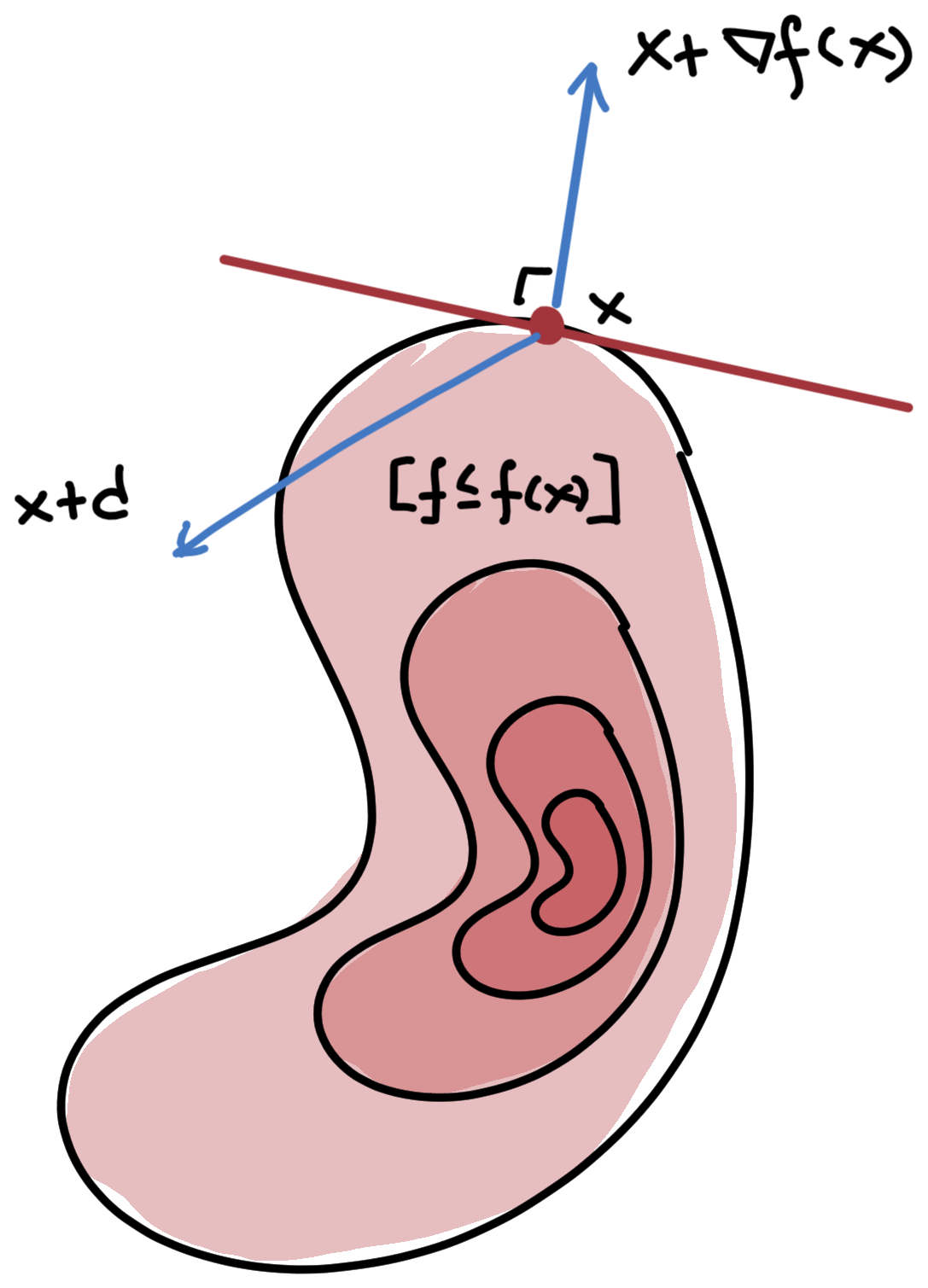
Definition 2 (Level set) The \(\alpha\)-level set of \(f\) is the set of points \(x\) where the function value is at most \(\alpha\):

\[ [f\leq \alpha] = \{x\mid f(x)\leq \alpha\} \]


A direction \(d\) points “into” the level set \([f\leq f(x)]\) if \[f'(x;d) = \nabla f(x)\T d < 0\]

Linear approximation

If \(f:\Rn\to\R\) is differentiable at \(x\), then for any direction \(d\) \[ \begin{aligned} f(x+d) &= f(x) + \nabla f(x)\T d + \omicron(\norm{d})\\ &= f(x) + f'(x;d) + \omicron(\norm{d}) \end{aligned} \] The remainder \(\omicron:\R_+\to\R\) decays faster than \(\norm{d}\)

\[\lim_{α\to0+}\frac{\omicron(α)}{α}=0\]


1st-order conditions

Theorem 2 (Necessary first-order conditions) For \(f:\Rn\to\R\) differentiable, \(x^*\) is a local minimizer only if it is a stationary point: \[ \nabla f(x^*) = 0 \]

proof

  • up to first order, for any direction \(d\) \[ \begin{aligned} f(x^*+\alpha d) - f(x^*) &= \nabla f(x^*)\T (\alpha d) + o(\alpha\|d\|)\\ &= \alpha f'(x^*;d) + o(\alpha\|d\|) \end{aligned} \]

  • because \(f\) is (locally) minimal at \(x^*\) \[ \begin{aligned} 0\le\lim_{\alpha\to 0^+}\frac{f(x^*+\alpha d) - f(x^*)}{\alpha} &= f'(x^*;d)=\nabla f(x^*)\T d \end{aligned} \]

  • because this holds for all \(d\), \(\nabla f(x^*)=0\)

Example: Quadratic

\[ f(x) = \tfrac{1}{2}x\T Hx - c\T x + \gamma, \quad H=H\T\in\Rn, \quad c\in\Rn \]

  • \(x^*\) is a local minimizer only if \(\nabla f(x^*)=0\), ie, \[ 0 = \nabla f(x^*) = Hx^* - c \quad\Longrightarrow\quad Hx^*=c \]

  • if \(\Null(H)\ne\emptyset\) and \(b\in\range(H)\), then there exists \(x_0\) such that \(Hx_0=b\) and \[ \argmin_x\, f(x) = \{\, x_0 + z \mid z\in\Null(H)\,\} \]

Example: Least squares

\[ f(x) = \tfrac{1}{2}\|Ax-b\|^2 = \tfrac{1}{2}(Ax-b)\T(Ax-b) = \tfrac{1}{2}x\T \underbrace{(A\T A)}_{=H}x - \underbrace{(b\T A)}_{=c\T}x + \underbrace{\tfrac{1}{2}b\T b}_{=\gamma} \]

  • \(x^*\) is a least-squares solution if (and only if) it satisfies the normal equations \[ 0 = \nabla f(x^*) = A\T Ax^* - A\T b \quad\Longleftrightarrow\quad A\T Ax^*=A\T b \]

Example: Nonlinear least squares

\[ f(x) = \tfrac{1}{2}\|r(x)\|^2 = \tfrac{1}{2}r(x)\T r(x) = \tfrac12\sum_{i=1}^m r_i(x)^2 \] where \[ r(x) = \begin{bmatrix} r_1(x)\\ \vdots\\ r_m(x) \end{bmatrix} \quad\text{where}\quad r_i:\Rn\to\R,\ i=1,\ldots,m \]

gradient

\[ \begin{aligned} \nabla f(x) = \nabla\left[\tfrac{1}{2}\sum_{i=1}^m r_i(x)^2\right] &= \sum_{i=1}^m \nabla r_i(x) r_i(x)\\ &= \underbrace{\begin{bmatrix} \, \nabla r_1(x) \mid \cdots \mid \nabla r_m(x)\, \end{bmatrix}}_{\nabla r(x)\equiv J(x)\T} \begin{bmatrix} r_1(x)\\ \vdots\\ r_m(x) \end{bmatrix} = J(x)\T r(x) \end{aligned} \]

Gradients and convergence

using Plots
using Optim: g_norm_trace, f_trace, iterations, LBFGS, optimize

f(x) = (1 - x[1])^2 + 100 * (x[2] - x[1]^2)^2

x0 = zeros(2) 
res = optimize(f, x0, method=LBFGS(), autodiff=:forward, store_trace=true)
fval, gnrm, itns = f_trace(res), g_norm_trace(res), iterations(res)
plot(0:itns, [fval gnrm], yscale=:log10, lw=3, label=["f(x)" "||∇f(x)||"], size=(600, 400), legend=:inside)