Regularized Least Squares
Regularization introduces to an optimization problem prior information or assumptions about properties of an optimal solution. A regularization parameter governs the tradeoff between the fidelity to the unmodified problem and the desired solution properties.
Slides
The Pareto frontier
The standard least-squares problem can be interpreted as a method for recovering some underlying object (say, a signal or image) encoded in the vector \(x_0\) using noisy measurements of the form \[ b := Ax_0 + \eta, \tag{1}\] where \(\eta\) is random additive error in the observations \(b\) and the matrix \(A\) describes the measurement process. The least-squares problem \[ \min_{x\in\Rn}\ \|Ax-b\|^2. \] seeks a solution \(x\) under the implicit assumption that the noise term \(\eta\) is small.
But what if \(x\) also needs to satisfy some other competing objective? Suppose, for example, that we have also available other set of measurements of \(x_0\) of the form \(d = Cx_0+w\), where \(w\) is also random error. The “best” choice for \(x\) is not necessarily Equation 1, and instead we wish to choose \(x\) to balance the two objective function values \[ f_1(x) \quad\text{and}\quad f_2(x). \tag{2}\]
Generally, we can make \(f_1(x)\) or \(f_2(x)\) small, but not both. Figure 1 sketches the relationship between the pair \(\xi(x):=\{f_1(x), f_2(x)\}\).
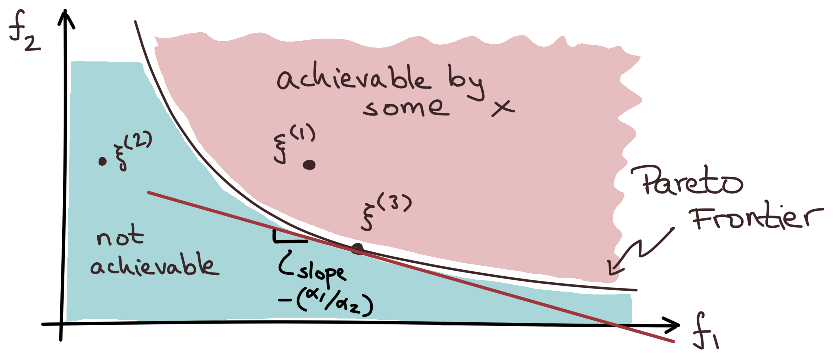
The objective pairs on the boundary of two regions is the Pareto frontier. We can compute these Pareto optimal solutions \(x\) by solving the optimization problem
\[ \min_x \{α₁f_1(x)+α_2 f_2(x)\,\}, \tag{3}\]
where the pair of positive penalty parameters \((\alpha_1,\alpha_2)\) provides the relative weight between the objectives.
For fixed penalties \(\alpha_1\) and \(α_2\), the set
\[ \{\ (f_1(x),f_2(x)) \mid α_1f_1(x) + α_2 f_2(x) = \alpha,\ x \in \R^n\ \} \]
forms the graph of a line with slope of \(-(α_1/α_2)\). We may visualize the optimization problem in Equation 3 as the problem of finding the smallest value \(\alpha\) such that the line is tangent to the Pareto frontier, as shown in Figure 1.
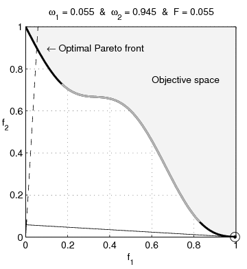
Figure 2 shows an example of a nonconvex Pareto frontier. In this case, the Pareto optimal solutions are not unique, and so the optimization problem Equation 3 may have multiple solutions.
Equation 3 is formulated using two penalty parameters, one for each objective. In general, we may have more than two objectives, and so we would need to introduce a penalty parameter for each objective. But in the particular case where we have only two objectives, we can equivalently formulate the problem using a single penalty parameter \(\lambda\):
\[ \min_x \{f_1(x) + \lambda f_2(x)\,\}, \tag{4}\]
with \(\lambda=α_2/α_1\). This is possible because multiplying the objective function by a positive constant does not change the location of the Pareto frontier.
Tikhonov regularization
A particularly common example of regularized least-squares is Tikhonov regularization, which has the form
\[ \min_{x} \half\|Ax-b\|^2 + \lambda\half\|Dx\|^2. \]
This objective can be expressed equivalently as
\[ \|Ax-b\|^2+\lambda\|Dx\|^2 = \bigg\|\begin{bmatrix}A\\\sqrt{\lambda}D\end{bmatrix} x - \begin{bmatrix}b\\ 0\end{bmatrix}\bigg\|^2. \]
If \(D\) has full column rank, then the stacked matrix \[ \begin{bmatrix}A\\\sqrt{\lambda}D\end{bmatrix} \] necessarily also has full rank for any positive \(\lambda\), which implies that the regularized problem always has a well-defined unique solution.
Example: Signal denoising
Consider a noisy measurement
\[ b := x^\natural + \eta \]
of a signal \(x^\natural\), where the vector \(\eta\) represents unknown noise, say, due to measurement error. Here’s a simple 1-dimensional noisy signal:
Code
The obvious least-squares problem
\[ \min_{x}\ \half\|x-b\|^2 \]
isn’t useful because the optimal solution is simply the noisy measurements \(b\), and so it doesn’t yield any new information. But suppose we believe that the signal is “smooth” in the sense that the consecutive elements of the vector \[ x=(x_1,\ldots,x_i,x_{i+1},\ldots,x_n)\] change relatively little, i.e., the difference \(|x_i-x_{i+1}|\) is small relative to \(x\). In this case, we might balance the least-squares fit against the smoothness of the solution by instead solving the regularized least-squares problem
\[ \min_{x}\ \half\underbrace{\vphantom{\sum_{i=1}}\|x-b\|^2}_{f_1(x)} + λ\half \underbrace{\sum_{i=1}^{n-1}(x_i - x_{i+1})^2}_{f_2(x)}. \tag{5}\]
The role of the regularizer \(f_2(x)\) is to promote smooth changes in the elements of \(x\).
Matrix notation
We can alternatively write the above minimization program in matrix notation. Define the \((n-1)\)-by-\(n\) finite difference matrix
\[ D = \begin{bmatrix} 1 & -1 & \phantom+0 & \cdots & \cdots & \phantom+0\\ 0 & \phantom+1 & -1 & 0 & \cdots & \phantom+0\\ \vdots & \ddots & \ddots & \ddots & & \vdots \\ \vdots & \cdots & \phantom+0 & 1 & -1 & \phantom+0\\ 0 & \cdots & & 0 & \phantom+1 & -1 \end{bmatrix} \] which when applied to a vector \(x\), yields a vector of the differences:
\[ Dx = \begin{bmatrix} x_1 - x_2 \\ x_2 - x_3 \\ \vdots \\ x_{n-1} - x_n \end{bmatrix}. \]
Then we can rephrase the regularization objective as \[ f_2(x) = \sum_{i=1}^{n-1}(x_i - x_{i+1})^2 = \|Dx\|^2. \] This allows for a reformulation of the weighted leas squares objective into a familiar least squares objective:
\[ \|x-b\|^2+\lambda\|Dx\|^2 = \bigg\| \underbrace{ \begin{bmatrix} I\\\sqrt{\lambda}D \end{bmatrix}}_{\hat{A}}x - \underbrace{ \begin{bmatrix}b\\ 0\end{bmatrix}}_{\hat{b}}\bigg\|^2. \]
So the solution to the weighted least squares minimization program {#eq-regularized_LS_identity} satisfies the normal equation \(\hat{A}\T\hat{A}x = \hat{A}\T\hat{b}\), which simplifies to
\[ (I + \lambda D\T D)x = b. \]
The following function generates the required finite-difference matrix using a sparse matrix data structure, which is more efficient than a dense matrix for large \(n\) because it only stores the nonzero entries:
Here’s an example of a small finite-difference matrix:
3×4 SparseArrays.SparseMatrixCSC{Float64, Int64} with 6 stored entries:
 1.0  -1.0    ⋅     ⋅
  ⋅    1.0  -1.0    ⋅
  ⋅     ⋅    1.0  -1.0
The function below returns a generator, which produces \(n\) logarithmically-spaced numbers in the interval \([x_1,x_2]\):
Now solve the regularized least-squares problem for several values of \(\lambda\in[1,10^4]\):
Code
Note that the expression  = [ I; √λ*D ] contains the UniformScaling object I from the LinearAlgebra package. It represents an identity matrix of any size, i.e., I is a shorthand for UniformScaling(1):
Equivalent constrained formulations
The formulation given in Equation 4 is an example of an additive penalty method, where the functions \(f_1\) and \(f_2\) are added together with balancing penalty parameter \(\lambda\). But there are other equally valid formulations that yield the same Pareto optimal solutions. For example, here are three related formulations:
\[ \begin{aligned} \min_x\,&\{f_1(x) + \lambda f_2(x)\,\}\\ \min_x\,&\{f_1(x)\mid f_2(x) \leq τ\} \\ \min_x\,&\{f_2(x)\mid f_1(x) \leq \sigma\} \end{aligned} \]
In the first formulation, the penalty parameter \(\lambda\) controls the tradeoff between the two objectives. The second and third formulations are constrained, and the parameters \(\tau\) and \(\sigma\) directly control the size of \(f_2(x)\) and \(f_1(x)\), respectively. Each formulation has its place in the context of an application, and the choice of formulation is often a matter of convenience.
Figure 4 shows the result the three formulations for a small instance of Tikhonov-type regularization, where \(f_1(x)=\|Ax-b\|^2\) and \(f_2(x)=\|x\|^2\). Each requires a different choice of penalty parameter \(\lambda\), \(\tau\), or \(\sigma\) to achieve the same solution, but the shape of the Pareto frontier is the same for all three formulations.