Pareto curve

The Pareto curve plays a central role in SPGL1. It is given as the lowest residual norm, as a function of $\tau$, which bounds the maximum allowable primal norm of the iterate $x$, i.e., $\|x\|_p\le\tau$.

Example Pareto curve (blue) along with a desired misfit level \(\sigma\) and Lasso parameter \(\tau\) that attains the desired solution.

Solving the Lasso problem for a given value of $\tau$ amounts to evaluating a point on the curve. The basis-pursuit denoise problem is more difficult: we are given $\sigma$ and need to find the value of $\tau$ where the values of the Pareto curve attains the desired value.

Root finding

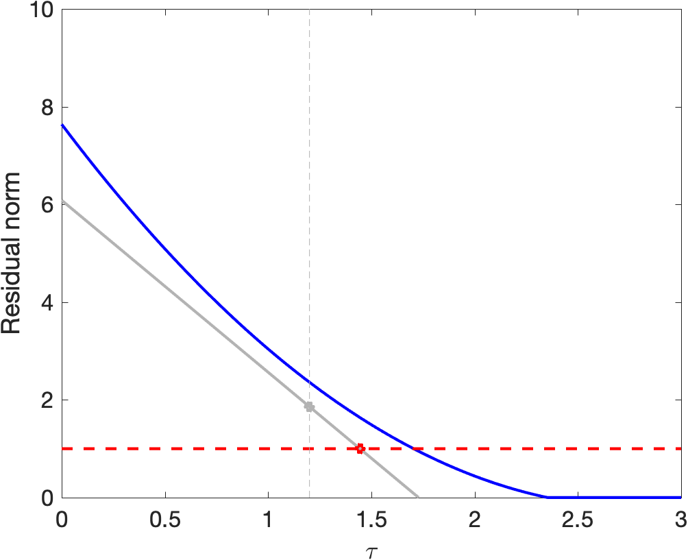
SPGL1 solves the basis-pursuit problem by solving a sequence of Lasso problems with different values of $\tau$. Given the solution of a Lasso problem, it determines the gradient of the Pareto curve at that point, which allows us to do root-finding. As an illustration, suppose we start at $\tau=0$ and solve the Lasso problem for this value (this always gives $x=0$). We then evaluate the gradient, which leaves us at the situation shown in the left plot below. We then update $\tau$ to the point where thelinear approximation to the Pareto curve intersect with the desired value of $\sigma$, indicated by the red dot. In this case this gives, say $\tau= 1.2$.

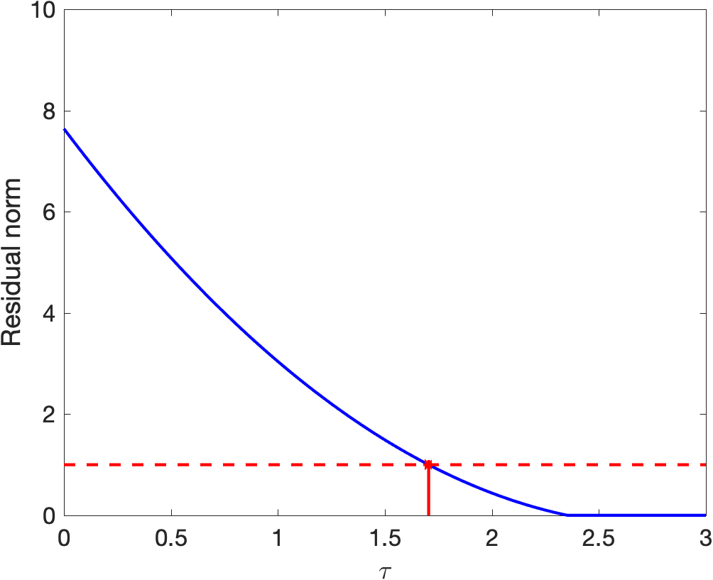
We then solve the Lasso problem with the new value of $\tau$, as shown in the right plot, and repeate the procedure until the solution has a residual norm that is sufficiently close to $\sigma$.

Implementation

SPGL1 provides options that control the root-finding process. The most important option, options.rootfindMode, specified whether root finding is done using the primal or the dual mode, with parameter values 0 and 1 respectively.

Primal mode

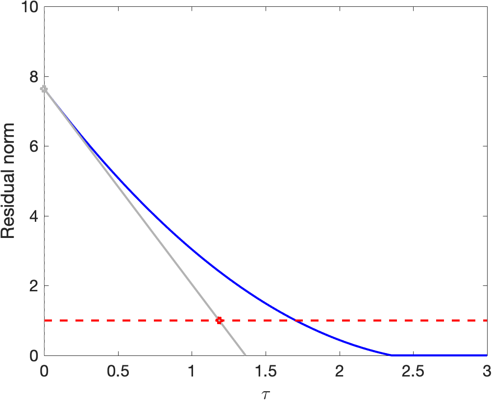
When using the primal objective, SPGL1 uses relaxed conditions to determine whether the Lasso subproblem is solved and approximates the gradient based on the primal objective. This root-finding mode can be very fast, but may result in value of $\tau$ that exceeds the minimum. As a result, this mode is useful when a quick solution is needed, or for large-scale problems where highly accurate solves of the subproblem are prohibitive. An exaggerated illustration of root-finding on the Pareto curve in the primal mode is given in the image below. The subproblem is solved approximately for $\tau=1.2$. The solution (indicated by the gray point) may be slighly above the Pareto curve, or the gradient may be too flat. This makes it possible to 'overshoot' the target and obtain a solution with a value $\tau$ that exceeds the minimum possible value.

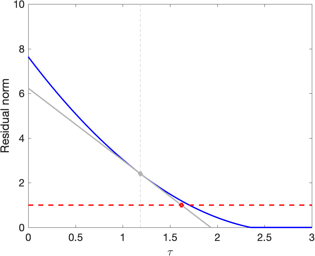
Dual mode

In the dual root-finding mode we apply root finding based on linear under-approximation of the Pareto curve. Provided that the initial $\tau$ is below the final value (a value of zero is always highly recommended), there is never any overestimation. As illustrated below, we use the dual objective value (indicated by the gray dot) along with a gradient to determine the next value of $\tau$. A new value for the intersection with the desired misfit level $\sigma$ is computed at every iteration and the maximum value is maintained for the next root-finding step. Root finding is initiated when the duality gap is a fraction (options.rootfindTol) of the difference between $\sigma$ and the primal objective. As the overall gap shrinks towards the solution, increasingly accurate solves are automatically enforced.